THE UNIVERSITY OF MARYLAND
UNIVERSITY COLLEGE
GRADUATE SCHOOL
A STUDENT RESEARCH REPORT
for
CSMN 658: Software Reliability and Reuseability
A Comparison of Two Software Reliability Engineering (SRE) Models:
Jelinski-Moranda and Musa-Okumoto Logarithmic Poisson
Michael J. Mangieri
December 7, 2000
Abstract
This paper will compare two popular software reliability models in use today: the Jelinski-Moranda model and the Musa-Okumoto model. An in-depth critical comparison is not possible in the amount of space available in this paper, but a reasonable attempt will be made to provide the reader with a general consensus of the basic differences and commonalities between the two models. The focus will be on specific attributes and qualities of the models, such as the form of their respective failure rate functions, the data inputs required to exercise the models, and the assumptions that must be true for the models to produce reliable and useful data. After a comparison of the models is presented, a short analysis of the differences in the resulting reliability predictions will be given.
A Comparison of Two SRE Models:
Jelinski-Moranda and Musa-Okumoto Logarithmic Poisson
Before a discussion of the main topic is presented, one may inquire why an analysis of software reliability is really necessary. After all, shouldn't software developers just remove as many defects in the code as possible before it is released as a product, thereby making the claim that the product is as reliable as possible?
This may not be desirable. First, the cost to remove the last remaining defect may be disproportionately expensive compared to the total cost spent on repairing all currently discovered defects. Second, removing x% of defects may not increase product reliability by x%. It may be a better business case to accept some level of unreliability and pay for future failure costs. This is one of the key decisions that must be made by the software project manager, and the use of reliability models helps to put a perspective on this problem. The following three questions are important: How reliable is the software currently? How much more testing is needed before the software can be released? Will the reliability requirements be satisfied in time to release the software? Indeed, the field of software reliability engineering is closely allied with and related to the amount of testing (Musa, 1984). With these three questions in mind, a comparison of two reliability models is presented.
Lyu (1996) points out that the failure process is dependent on three principal factors: fault introduction, fault removal and the operational environment. A software reliability model specifies the general form of this dependence. Both the Jelinski-Moranda and Musa-Okumoto models are recommended by the AIAA (Paulson, 1998). Both are widely used and commonly accepted. Of the two, Jelinski-Moranda is more popular and well known. The Musa-Okumoto model is widely accepted in the telecommunications environment (Paulson, 1998). The Jelinski-Moranda model's metrics are readily available and easily collected. Musa-Okumoto allows significant changes to the software while testing and reliability evaluation takes place.
Musa (1999) makes the point that a good reliability model must possess a number of important characteristics. It must give a good projection of future failure behavior. The quantities it produces must be useful to the organization using the model. It must be simple, not confusing to the analyst. It should be widely applicable. The model must be based on sound assumptions. Both of these models possess all these attributes.
Categorization of models
Musa and Okumoto (1983) categorize the Jelinski-Moranda model as belonging to the Exponential class, with Binomial type. The Musa-Okumoto model belongs to the Geometric family and is Poisson in type. Since the Musa-Okumoto model belongs to a family, it assumes an infinite number of failures are inherent in the subject system. The functional form of the failure intensity is in terms of the expected number of failures experienced. This model is categorized by failures per time period. The Jelinski-Moranda model belongs to a class, and so it assumes a finite number of failures are present. The functional form of it's failure intensity is in terms of time. This model is categorized by time between failures (Musa, 1999).
Assumptions
There are three basic assumptions that are common to both models (Farr, 1996a), and these are known as the Standard Assumptions:
1. The software is operated in a way that can be mapped to the reliability predictions (model estimates derived can be used in the environment that the predictions are desired).
2. Every fault, of a specific severity class, has an equal chance of occurring.
3. Failures, when faults are detected, are independent.
In addition to the standard assumptions, Jelinski-Moranda has the following assumptions:
1. Errors occur by accident.
2. Failure rate is proportional to the number of remaining defects.
3. Failure rate remains constant over the intervals between fault occurrences.
4. Faults are corrected instantaneously and perfectly – no new faults are introduced.
Likewise, the Musa-Okumoto model has specific assumptions as well. They are, again in addition to the standard assumptions:
1. Failure intensity decreases exponentially with the expected number of failures experienced.
2. The cumulative number of failures follows a Poisson process.
It is important that these assumptions be taken seriously. In fitting any model to a given set of data, the accuracy of the predictions are only as good as the appropriateness of the model chosen.
Data requirements
The data requirements for both models are the same and simple in concept. There are two parameters, only one of which is needed. One is the elapsed time between failures. The other is the actual times that the software failed. Both models use execution time. Musa (1999) points out that only the Musa basic and Musa-Okumoto models are explicitly defined as being in the execution time domain. All others are either calendar time models or their domains are not explicitly stated.
Comparisons
In light of the questions earlier in this paper, each of the two models presented for comparison here provide a good mechanism for future predictions of software faults, and hence, a reliability estimation. These predictions can be used to adjust resource allocations and schedule testing time. Both of these models perform fairly well in this regard. However, Farr (1996b) clearly points out that software, under reliability evaluation of these models, "… must have matured to the point that extensive changes are not being routinely made".
The Jelinski-Moranda (J-M) model is one of the earliest proposed, often called the de-eutrophication model. It was developed by two McDonnell Douglas employees, Jelinski and Moranda, while working on a few Navy projects. The rate of fault detection is directly proportional to the current fault content of the software. The hazard rate of the J-M model is best expressed as shown in equation 1. This clearly shows that the failure rate decreases proportionally with the
|
|
(1) |
parameter ![]() , called the
proportionality constant and shows a per-fault constant hazard rate. N
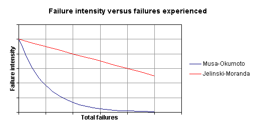
represents the total number of faults in the software. Figure 1 shows graphically how the rate decreases as faults
are discovered. Although the plot is shown as a continuous function, in reality
the hazard rate is a step function since improvements in reliability only take
place when a failure is fixed. The hazard rate decreases by
, called the
proportionality constant and shows a per-fault constant hazard rate. N
represents the total number of faults in the software. Figure 1 shows graphically how the rate decreases as faults
are discovered. Although the plot is shown as a continuous function, in reality
the hazard rate is a step function since improvements in reliability only take
place when a failure is fixed. The hazard rate decreases by ![]() every time a fault is
fixed.
every time a fault is
fixed.
|
Figure 1 - Failure intensity versus failures |
The Musa-Okumoto (M-O) model demonstrates a hazard rate that is exponential in nature, as shown in equation 2, and is a continuous function.
|
|
(2) |
In this case, the hazard rate is
not constant, but decreases exponentially as failures occur (see Figure 1). The parameter ![]() , is called the failure intensity decay parameter. It
indicates the magnitude of the failure rate change with respect to faults. In
this model, the hazard rate is controlled by an initial rate modified by an
exponential decay as determined by the decay parameter
, is called the failure intensity decay parameter. It
indicates the magnitude of the failure rate change with respect to faults. In
this model, the hazard rate is controlled by an initial rate modified by an
exponential decay as determined by the decay parameter ![]() . The M-O model is called logarithmic since the expected
number of failures over time is a logarithmic function (as can be seen by
plotting the natural logarithm of failure intensity over mean failures as Musa
(1999) suggests). One of the important key points to remember is that in the
J-M model, fixes contribute to the overall reliability, whereas in the M-O
model, they do not have any direct effect on reliability.
. The M-O model is called logarithmic since the expected
number of failures over time is a logarithmic function (as can be seen by
plotting the natural logarithm of failure intensity over mean failures as Musa
(1999) suggests). One of the important key points to remember is that in the
J-M model, fixes contribute to the overall reliability, whereas in the M-O
model, they do not have any direct effect on reliability.
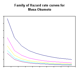
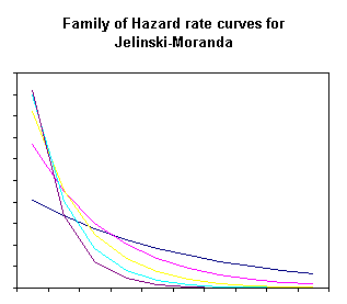
In both models, the value of the decay parameter ![]() controls the shape of
the resultant hazard rate curve. Although Figure
1 shows no cross of model lines, this is not always the
case. Figure 2 and Figure
3 show the family of curves that can arise from varying
values of the decay parameter.
controls the shape of
the resultant hazard rate curve. Although Figure
1 shows no cross of model lines, this is not always the
case. Figure 2 and Figure
3 show the family of curves that can arise from varying
values of the decay parameter.
|
Figure 2 – Musa-Okumoto family of curves |
|
Figure 3 – Jelinski-Moranda family of curves |
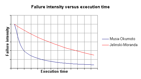
In order to examine these two models more closely, the analysis is moved to a time domain viewpoint. The two models possess different failure intensity functions, as expected. Equations 3 and 4 represent the failure intensity functions for the J-M and M-O models respectively. Figure 4 shows a sample failure intensity plot with respect to execution time.
|
|
(3) |
|
|
(4) |
|
Figure 4 - Failure intensity versus execution time |
The M-O model shows a fairly rapid decrease in failure rate in the early period of execution while the J-M model shows a failure rate that remains high for a much longer period. Later, the M-O curve flattens and the decrease rate is very slow. The exponential rate of decrease in the M-O model indicates that earlier discoveries of failures have a greater impact on reducing the failure intensity function than those found later (Farr, 1996c).
|
|
(5) |
|
|
(6) |
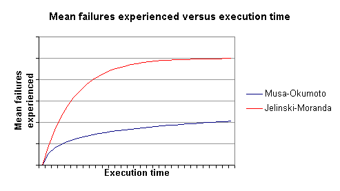
Finally, the cumulative failure function (mean value function) for each of the models are given in equation 5 for J-M and equation 6 for M-O. They represent how failures accumulate over time.
Figure 5 shows a representation of the cumulative number of failures predicted by each model. Notice the flattening of the J-M curve indicative of a finite failure model.
|
Figure 5 - Mean failures experienced versus execution time |
One of the questions at the start of this paper proposed a
possible goal of a software development firm. That is, to determine when
sufficient testing has been completed on a software system so it can be
released with a known reliability evaluation. In regards to the M-O model, this
can be answered through use of equation 7. ![]() is the initial
failure intensity,
is the initial
failure intensity, ![]() is the required
failure intensity
is the required
failure intensity
|
|
(7) |
(value desired before product is deemed ready to release), ![]() is the intensity
decay parameter and
is the intensity
decay parameter and ![]() the elapsed execution
time. Once the value of
the elapsed execution
time. Once the value of ![]() is determined and the
remaining parameters entered, the result of the calculation yields the amount
of further execution time required to achieve the required failure intensity.
Although specific to the M-O model it illustrates the usefulness of software
reliability engineering in answering the question "how much more testing
is necessary …" (Paulson, 1998).
is determined and the
remaining parameters entered, the result of the calculation yields the amount
of further execution time required to achieve the required failure intensity.
Although specific to the M-O model it illustrates the usefulness of software
reliability engineering in answering the question "how much more testing
is necessary …" (Paulson, 1998).
Reliability considerations
In discussing the reliability predictions of the two models Musa (1999) reminds us that reliability is dependent not only on the failure intensity but also on the period of execution time. As the period of time increases, the reliability of the system decreases.
The Musa-Okumoto model clearly shows a tendency to produce
low MTTF values in the initial period of software test, as the failure
intensity function is very steep in the early execution time periods (MTTF is
approximated by the inverse of the failure rate). Farr (1996d) recommends this
model for systems that are likely to have operational profiles that are
non-uniform to a great degree. After the initial period of shakeout, the MTTF
values will increase rapidly. Since the reliability ![]() of a system is a
function of the cumulative density function
of a system is a
function of the cumulative density function ![]() as shown in equation
8, and since
as shown in equation
8, and since ![]() is the integral of
is the integral of ![]() over time,
over time, ![]() is essentially given
by equation 9. Based on this relationship, reliability values
is essentially given
by equation 9. Based on this relationship, reliability values
|
|
(8) |
|
|
(9) |
(MTTF) for M-O are very good later on in the testing phase as the
curve of ![]() flattens
dramatically.
flattens
dramatically.
Jelinski-Moranda follows a more gradual reliability improvement curve as the MTTF values tend to remain rather constant, although decreasing with execution time. This is to be expected as J-M assumes a fixed number of faults in the system.
Conclusion
A very general comparative analysis of two software reliability models, the Musa-Okumoto model and Jelinski-Moranda model, has been described. Both are acceptable models and are recommended for use provided they are used properly. Software modifications, not fixes, must be completed for these models to produce reasonable predictions of reliability.
References
Farr, W. (1996a). Software Reliability Modeling Survey. In M. R. Lyu (Ed.), Handbook of Software Reliability Engineering (p. 78). New York: McGraw-Hill.
Farr, W. (1996b). Software Reliability Modeling Survey. In M. R. Lyu (Ed.), Handbook of Software Reliability Engineering (p. 77). New York: McGraw-Hill.
Farr, W. (1996c). Software Reliability Modeling Survey. In M. R. Lyu (Ed.), Handbook of Software Reliability Engineering (p. 102). New York: McGraw-Hill.
Farr, W. (1996d). Software Reliability Modeling Survey. In M. R. Lyu (Ed.), Handbook of Software Reliability Engineering (p. 104). New York: McGraw-Hill.
Lyu, M. R. (1996). Software Reliability Modeling Survey. In M. R. Lyu (Ed.), Handbook of Software Reliability Engineering (p. 18). New York: McGraw-Hill.
Musa, J. D. (1984). Software Reliability. In C. R. Vick, & C. V. Ramamoorthy (Eds.), Handbook of Software Engineering (p. 393). New York: Van Nostrand Reinhold Company.
Musa, J. D. (1999). Software Reliability Engineering. New York, New York: McGraw-Hill.
Musa, J. D., & K. Okumoto (1983). Software Reliability Models: concepts, classification, comparisons, and practice. In J. K. Skwirzynski (Ed.), Electronic systems effectiveness and life cycle costing, NATO ASI Series (pp. 395-424). Heidelberg: Springer-Verlag.
Paulson, J. and Yue, T. (1998). Software Reliability Measurement Plan for CellTel Ltd. [Online]. Available: http://cern.ucalgary.ca/~paulson/SENG623/MetricsPlan/metricsplan.html
Bibliography
Farr, W. (1996). Software Reliability Modeling Survey. In M. R. Lyu (Ed.), Handbook of Software Reliability Engineering (p. 78). New York: McGraw-Hill.
Fenton, N. E., & Neil, M. (1999). A Critique of Software Defect Prediction Models. IEEE Transactions on Software Engineering, 25, 675-687.
Grams, T. (1999). Reliability Growth Models Criticized.
[Online]. Available:
http://www.fh-fulda.de/~fd9006/RGM/RGMcriticized.html
Hecht, M, Tang, D., & Hecht, H. (1996). Software
Reliability Assessment – Myth and Reality. [Online]. Available:
http://appl.nasa.gov/library/docs/issues12/inppm12h.htm
Lanubile, F. & Visaggio, G. (1997). Evaluating predictive quality models derived from software measures: lessons learned. The Journal of Systems and Software, 38, 225-234.
Littlewood, B. (2000). Problems of Assessing Software
Reliability. [Online]. Available:
http://www.csr.city.ac.uk/people/bev.littlewood/bl_public_papers/SCSS_2000/SCSS_2000.pdf
Lyu, M. R. (1996). Software Reliability Modeling Survey. In M. R. Lyu (Ed.), Handbook of Software Reliability Engineering (p. 18). New York: McGraw-Hill.
Musa, J. D. (1984). Software Reliability. In C. R. Vick, & C. V. Ramamoorthy (Eds.), Handbook of Software Engineering (p. 393). New York: Van Nostrand Reinhold Company.
Musa, J. D. (1999). Software Reliability Engineering. New York, New York: McGraw-Hill.
Musa, J. D., & K. Okumoto (1983). Software Reliability Models: concepts, classification, comparisons, and practice. In J. K. Skwirzynski (Ed.), Electronic systems effectiveness and life cycle costing, NATO ASI Series (pp. 395-424). Heidelberg: Springer-Verlag.
Nour, P. & Mehrotra, R. (2000). Software Reliability and Testing CASRE Report. [Online]. Available: http://sern.ucalgary.ca/~philip/Seng/Seng609.11/Report.html
Paulson, J. and Yue, T. (1998). Software Reliability Measurement Plan for CellTel Ltd. [Online]. Available: http://cern.ucalgary.ca/~paulson/SENG623/MetricsPlan/metricsplan.html
Vouk, M. A. (2000). Software Reliability Engineering.
Wallace, D. R., Ippolito, L. M., and Cuthill, B. (1996).
Reference Information for the Software Verification and Validation Process.
[Online]. Available:
http://hissa.ncsl.nist.gov/HHRFdata/Artifacts/ITLdoc/234/val-proc.html
Wood, A. (1996). Predicting Software Reliability. Computer, 29(11), 69-77.
